OMDEC - Optimal Maintenance Decisions Inc.

Reliability continuous improvement – (Living RCM)

A Reliability Continuous Improvement Procedure applies processes and tools that support good maintenance decisions. The procedure provides confidence in protecting revenue from losses due to equipment failure. Business risk guides decision making. In physical asset management, risk can be defined as:

Risk = Consequences of failure X probability of failure

We define “failure” as the complete or partial loss of a required function. The Reliability Continuous Improvement Procedure mitigates risk by lessening the consequences of failure and / or by reducing its probability. The consequences of failure include:

Consequences of Failure =

Cost of repair + Lost revenue while out of service + Lost opportunity + Penalties as a result of safety and environmental violations + Lost reputation

The overall monetary consequences of failure often exceed the overall cost of preventive measures. Maintenance information systems should expose these costs on an annualized basis over a reasonable time horizon so that managers may consider them in their continuous review of policies and procedures. Typically maintenance information systems do not report such information routinely nor clearly. Managers must request specially prepared reports and analyses that consume significant engineering time and resources. Often in the heat of operations such analyses are overlooked. The Reliability Continuous Improvement Procedure addresses that issue and ensures that all relevant reporting needed for analysis is performed routinely and, for the most part, automatically. The second risk factor, failure probability (technically, the conditional failure probability), must, as well be accounted for in decisions and maintenance policy. Predicting the remaining useful life (RUL) of an asset requires specialized procedures and tools. These methods rely on good data. The Reliability Continuous Improvement Procedure ensures that correct data supports the decision process.

Probabilty of Failure: estimated by applying appropriate reliability analysis techniques to relevant data

Relevant data sources for continuous reliability decision support are:

1. Prior work orders (What failure modes (causes) have occurred or potentially occurred?),
2. Prior condition monitoring data (What monitored data patterns preceded failure or potential failure?),
3. Current operational and condition monitoring data (What is the appropriate course of action now?).

Reliability analysis of 1 and 2 provides decision models for acting upon 3. Reliability analysis requires that work order events (failures, potential failures, and suspensions) be considered together with observations preceding those events. The Reliability Continuous Improvement Procedure unifies these data sources for analysis.

Figure 1 The components of Reliability continuous improvement procedure

The Reliability Continuous Improvement Procedure incorporates “Living RCM” (LRCM) methods. LRCM ensures that historical work order data feeds reliability analysis software. LRCM promotes collaboration in updating the reliability knowledge base. A reliability knowledge base consists of knowledge records. Each knowledge record describes a required function, a functional loss description, a cause, effects (what happens), and its consequences (how does it matter). The Reliability Continuous Improvement Procedure will ensure the consistent compilation of reliability knowledge. The procedures will require that each significant work order, at closure, will reference a knowledge record in the knowledge base. As a result of this requirement, the work order becomes an instance of a knowledge record. Work orders define failure mode life cycles by marking their beginnings and endings. Reliability analysis “counts” instances of failure modes in a variety of ways. These include, for example Pareto analysis, Weibull analysis, Trend analysis, Top 10 analysis and numerous others. Reliability analysis, as depicted in Figure 1, generates “Good Engineering, Maintenance, & Reliability Practices” By amalgamating core asset management databases, the Reliability Continuous Improvement Procedure ensures that the team can perform reliability analysis. From these analyses they re-evaluate the tasks currently associated with a failure cause in the knowledge base. At the opportunity afforded by the work order closure activity, they determine what changes, if any, must be made to the knowledge record and, further, what changes must be undertaken to mitigate, to the degree required, the consequences of failure. The insights gained through reliability analysis lead the engineer to cost reduction and reliability improvement by optimizing maintenance policies.

Examples of reliability analysis:

1. CBM decision optimization

The engineer examines the incidences of a failure mode together with condition monitoring data preceding those failure events. Through statistical correlation analysis he will discover predictive patterns in the CM data (if they exist) for optimal decision making. Figure 2 applies an optimized maintenance decision. Figure 3 provides failure probabilities and confidence intervals.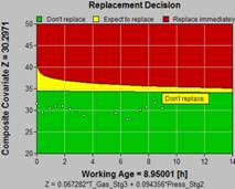

Figure 2 Optimal CBM decision

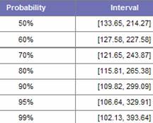Figure 3 Failure probability in intervals

2. Capital replacement decision optimization

From an analysis of the replacement costs and the repair costs of a fleet of capital items subject to periodic replacement the engineer can calculate an annualized cost for various replacement scenarios. The lowest annualized cost, represents the optimal economic replacement age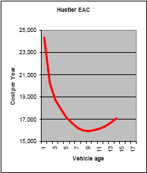

Figure 3 optimal replacement age

3. Simulation accuracy

The Reliability Continuous Improvement Procedure updates parameters used in simulation models for predicting equipment availability. LRCM ensures that decisions from simulation studies can benefit from the latest data as recorded in the CMMS.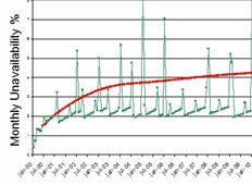

Figure 4 Projected unavailability

4. Risk Assessment (Criticality analyses)

The MTBF component of Risk Assessment will be updated automatically as new data is recorded in the CMMS. Continuous review of risk will be integrated with the reliability knowledge management process triggered at work order closure.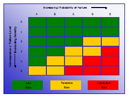

Figure 5 Risk matrix

5. Priority analysis

The Jackknife plot places failure modes that have occurred in a specified time period on a logarithmic grid. The vertical axis measures severity, for example downtime. The horizontal axis measures frequency. The failure modes that fall in the red region require immediate managerial attention. The Reliability continuous improvement procedure monitors the desired movement of failure modes towards the orgin.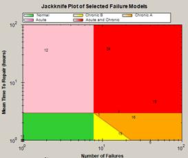

Figure 6 Jackknife (scatter chart) for priority analysis

 

6. Failure rate (Weibull) analysis

 

The age reliability relationship can be expressed in many ways. Figure 6 illustrates the failure rate (hazard rate). It is the probability of failure in the next relatively short time interval since the last renewal of the item. This analysis answers the questions: Is preventive maintenance technically feasible? Is there a materials quality or installation problem? What is the “useful life” of the item? Is the MTBF (reliability) of a randomly failing item acceptable?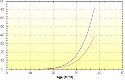

Figure 6 Weibull (failure rate) analysis

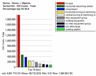
7. Top 10 analysis

Find the failure causes with the greatest impact on profitability in any class category or group and in any time window.

Figure 7 Top 10 analysis

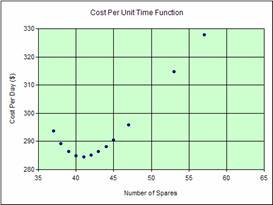
8. Spares analysis

A critical issue in spares management is to establish an appropriate level for insurance of an emergency spare whenever a critical long-life component fails. Such components would include transformers in an electrical utility or electric motors in a conveyor system. The question to be addressed is: "How many critical spares should be stocked?"

Figure 8 Spares analysis